【python因果库实战31】LaLonde 数据集匹配2

这里写目录标题使用匹配来估计结果并为 IPW 准备数据结论使用匹配来估计结果并为 IPW 准备数据我们这里有一些担忧即治疗组和对照组之间的数据可能过于不平衡以至于无法进行可靠的推断。虽然原则上倾向得分加权可以纠正协变量的不平衡但我们在这里看到这个数据存在一些相当严重的正则性positivity违反情况。当我们通过匹配数据进行条件化处理之后再使用逆概率加权IPW我们发现 IPW 在判断加权后的协变量不平衡方面更为有效。最有趣的是一旦协变量达到平衡效果的符号就会发生变化。我们先从使用单一邻居和有放回抽样的简单倾向得分匹配的结果开始看起。我们使用PropensityTransformer对象来计算倾向得分并将其添加到用于匹配的协变量中。fromcausallib.estimationimportIPW,Matchingfromcausallib.preprocessing.transformersimportPropensityTransformerfromsklearn.linear_modelimportLogisticRegressionimportpandasaspddeflearner():returnLogisticRegression(solverliblinear,max_iter5000,class_weightbalanced)如我们在 Faiss 笔记本中所展示的使用 Faiss 后端进行匹配要快得多。这需要安装 faiss-gpu 或 faiss-cpu。如果可用我们会自动选择 Faiss 后端否则会退回到 “sklearn”。try:fromcausallib.contrib.faissknnimportFaissNearestNeighbors knn_backendFaissNearestNeighborsexceptImportError:knn_backendsklearnpropensity_transformPropensityTransformer(include_covariatesFalse,learnerlearner())matcherMatching(propensity_transformpropensity_transform,with_replacementTrue,n_neighbors1,knn_backendknn_backend)matcher.fit(X,a,y)matcher.match(X,a)一种更好地理解我们的样本之间接近程度的方法是检查我们发现的匹配项的协变量。我们可以通过get_covariates_of_matches函数做到这一点。best_control_matchesmatcher.get_covariates_of_matches(1,0,X)best_treatment_matchesmatcher.get_covariates_of_matches(0,1,X)我们可以查看最差的匹配并看看哪些协变量没有匹配上。get_covariates_of_matchesDataFrame 包含了匹配项的协变量以及匹配的详细信息。这里我们将关注 “delta” 列best_control_matches.sort_values((match,distance),ascendingFalse)[delta].head(10)我们看到 1974 年和 1975 年的收入 (“re74” 和 “re75”) 以及年龄的匹配非常糟糕尽管其他协变量看起来匹配得相当好。我们可以同样地查看每个治疗样本找到的最佳匹配。我们发现匹配得更好无论是从倾向得分的距离还是从协变量来看。在这里收入的 delta 大约是我们从另一个方向得到的值的一个数量级小。best_treatment_matches.sort_values((match,distance),ascendingFalse)[delta].head(10)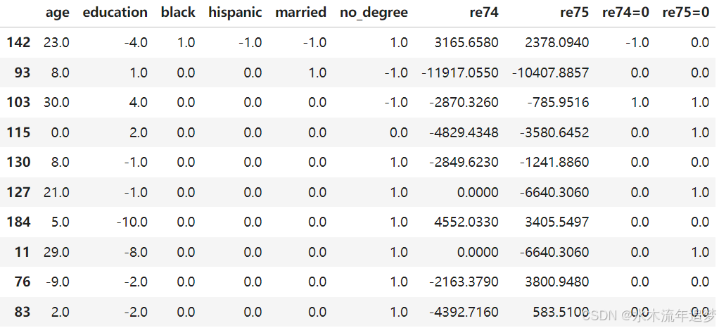这告诉我们对于每一个接受了就业培训的个体即治疗个体都有一个未接受治疗但非常相似的个体但是有许多控制组个体的协变量特别是收入水平与他们最近邻的治疗组个体大不相同。 我们可以通过进一步检查匹配控制样本和匹配治疗样本的倾向距离分布来探索这一观察结果。 pythonfrommatplotlibimportpyplotasplt f,axesplt.subplots(1,2,figsize(16,5))best_control_matches.match.distance.hist(axaxes[0],bins40)best_treatment_matches.match.distance.hist(axaxes[1],bins40)axes[0].set_xlabel($\Delta$ Propensity of closest match)axes[1].set_xlabel($\Delta$ Propensity of closest match)axes[0].set_ylabel(Count)axes[1].set_ylabel(Count)axes[0].set_title(Control)axes[1].set_title(Treatment)axes[0].axvline(xbest_treatment_matches.match.distance.max(),colorred,labelmax $\Delta$ propensity of treatment-control)axes[0].legend();哇当我们从治疗组寻找最近邻时找到的最大距离位于从控制组到治疗组最近邻距离的前几个百分位数内。实际上它正好位于第 6 百分位数内sum((best_control_matches.match.distancebest_treatment_matches.match.distance.max()))/len(best_control_matches)0.07171205693170932在这种情况下匹配如何帮助我们一方面我们可以做一个简单的、无放回的匹配并比较治疗组的配对来估计结果matcher.with_replacementFalsematcher.match(X,a)matcher.estimate_population_outcome(X,a)0.05093.4929421.06349.143530dtype:float64这样给我们带来了接受治疗者 $1752 的效果。这是非常显著的并且与直观的估计完全不同直观估计是负数。但我们只使用了原始数据集中大约 21,000 个样本中的 370 个。如果能更多地利用我们拥有的数据就更好了。我们可以做的一件事是使用卡尺并使用匹配来估计潜在结果importnumpyasnp matcher.n_neighbors3results,sample_count[[],[]]cvecnp.logspace(-7,-0.5,10)forcaliperincvec:matcher.calipercaliper matcher.with_replacementTruematcher.match(X,a)results.append(matcher.estimate_population_outcome(X,a))sample_count.append(matcher.samples_used_)cresultspd.DataFrame(dataresults,indexcvec)f,axesplt.subplots(1,2,figsize(16,7))axes[0].loglog(cvec,sample_count)axes[0].legend([control samples,treatment samples])axes[0].axhline(ysum(a0),ls:,colorC0)axes[0].axhline(ysum(a1),ls:,colorC1)axes[0].set_xlabel(caliper)axes[0].set_ylabel(sample count)axes[0].axis(tight)axes[1].semilogx(cvec,results)axes[1].legend([control prediction,treatment prediction])axes[1].set_xlabel(caliper)axes[1].set_ylabel(Expected Income)plt.tight_layout();这很有趣。我们看到这样我们可以使用一个滑动标度来调整匹配的严格程度随着我们纳入远距离匹配效果估计发生了显著变化即效果的符号发生了改变那么逆概率加权呢倾向得分是一个平衡权重只要我们解决了正则性问题我们应该能够以这种方式获得相当稳健的估计。我们甚至可以跟踪协变量的平衡情况看看我们在纠正正则性问题方面的表现如何。因为如果有正则性问题协变量将不能通过逆概率权重实现平衡。为了给 IPW 模型提供更多的数据我们可以扩展到三个邻居如果卡尺允许的话。fromcausallib.preprocessing.transformersimportMatchingTransformerfromcausallib.evaluation.metricsimportcalculate_covariate_balance caliper_vecnp.logspace(-5.5,-1,10)covbal[]n_neighbors3defmatch_then_ipw_weight(caliper):mtMatchingTransformer(propensity_transformPropensityTransformer(include_covariatesFalse,learnerlearner()),calipercaliper,n_neighborsn_neighbors)mt.fit(X,a,y)Xm,am,ymmt.transform(X,a,y)ipwIPW(learnerlearner())ipw.fit(Xm,am,)ipw_weightsipw.compute_weights(Xm,am)ipw_outcomeipw.estimate_population_outcome(Xm,am,ym)matched_treatedsum(am1)matched_controlsum(am0)covbalancecalculate_covariate_balance(Xm,am,ipw_weights)return{caliper:caliper,n_treated:matched_treated,n_control:matched_control,ipw_weights:ipw_weights,ipw_outcome:ipw_outcome,covariate_balance:covbalance.drop(columnsunweighted)}results[match_then_ipw_weight(c)forcincaliper_vec]covbal_dfpd.concat([i[covariate_balance]foriinresults],axis1)importseabornassbimportmatplotlib.pyplotasplt covbal_df.columns[%.6f%iforiincaliper_vec]covbal_noedu_dfcovbal_df.drop(labels[iforiincovbal_df.indexifeducationini])f,axplt.subplots(2,2,figsize(13,12))ax[0,0].errorbar(caliper_vec,covbal_noedu_df.mean(),yerrcovbal_noedu_df.std())ax[0,0].set_xscale(log)ax[0,0].set_xlabel(caliper)ax[0,0].set_ylabel(mean covariate balance)ax[0,1].semilogx(caliper_vec,[i[n_control]foriinresults],labelcontrol)ax[0,1].semilogx(caliper_vec,[i[n_treated]foriinresults],labeltreatment)ax[0,1].set_ylabel(sample count)ax[0,1].set_xlabel(caliper)ax[0,1].set_xscale(log)ax[0,1].set_yscale(log)ax[0,1].legend()ax[1,0].semilogx(caliper_vec,[i[ipw_outcome][0]foriinresults],labelcontrol)ax[1,0].semilogx(caliper_vec,[i[ipw_outcome][1]foriinresults],labeltreatment)ax[1,0].set_ylabel(outcome)ax[1,0].set_xlabel(caliper)ax[1,0].set_xscale(log)ax[1,0].legend()sb.heatmap(datacovbal_noedu_df,axax[1,1])ax[1,1].set_xlabel(caliper)plt.tight_layout();结论我们看到当扩展数据以包括非精确匹配时预测保持相对稳健直到一定程度。没有任何数据过滤的情况下IPW 因正则性问题而受到影响无法成功平衡协变量特别是之前的收入以及西班牙裔群体。因此尽管 IPW 方法具有强大的能力但它本身无法检测正则性问题并且可以通过使用匹配或类似程序进行过滤来改进。


:创建技能)


